This post is one in a series about GANce

In collaboration with Won Pound for his forthcoming album release via minaret records I was recently commissioned to lead an expedition into latent space, encountering intelligences of my own haphazard creation.

A word of warning:

This and subsequent posts as well as the GitHub etc. should be considered toy projects. Development thus far has been results-oriented, with my git HEAD following the confusing and exciting. The goal was to make interesting artistic assets for Won’s release, with as little bandwidth as possible devoted to overthinking the engineering side. This is a fun role-reversal, typically the things that leave my studio look more like brushes than paintings. In publishing this work, the expected outcome is also inverted from my typical desire to share engineering techniques and methods; I hope my sharing the results shifts your perspective on the possible ways to bushwhack through latent space.

So, with that out of the way the following post is a summary of development progress thus far. Here’s a demo:

There are a few repositories associated with this work:

• GANce, the tool that creates the output images seen throughout this post.
• Pitraiture, the utility to capture portraits for training.

If you’re uninterested in the hardware/software configurations for image capture and GPU work, you should skip to Synthesizing Images.

Background

thispersondoesnotexist.com will explain to you what StyleGAN does faster than words can. Serving as Won’s (and later my own) introduction introduction into the technology, it was particularly interesting to see results where the AI made a “mistake”.

These otherworldly portraits are easy to come by if you refresh the page enough times. The artifacts look like heavily synthesized but still reasonably passable at a glance.

Digging in a bit, it was a welcome surprise to see that the underlying source code of StyleGAN was written in Python. Python’s a favorite language as longtime readers will know. Seeing example training runs as posted on the Artificial Images YouTube channel made the training process seem approachable. Encouraged, I continued researching. The most natural entry-point into understanding how StyleGAN works is Making Anime Faces With StyleGAN by Gwern Branwen. This fabulous post goes over everything one could want to learn about and more, and concludes with a mountain of references.

As quickly as possible, the process for creating a StyleGAN (versions 1 and 2, things might be different in version 3 which was released during the development of this project.) network is as follows:

1. Create a large dataset of somewhat similar images.
2. Process the images such that they’re in an acceptable format for training (cropped, etc).
3. Train the network.

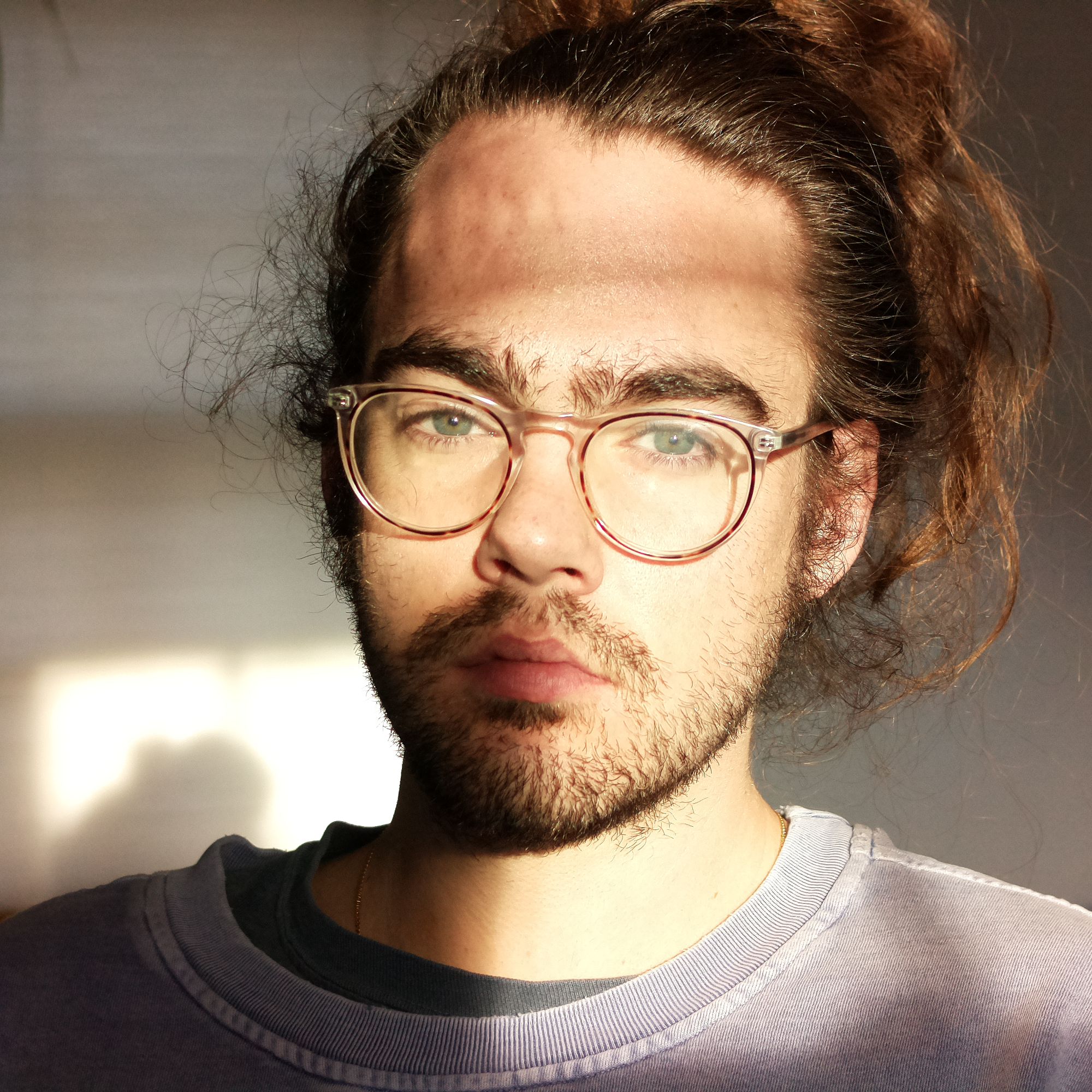
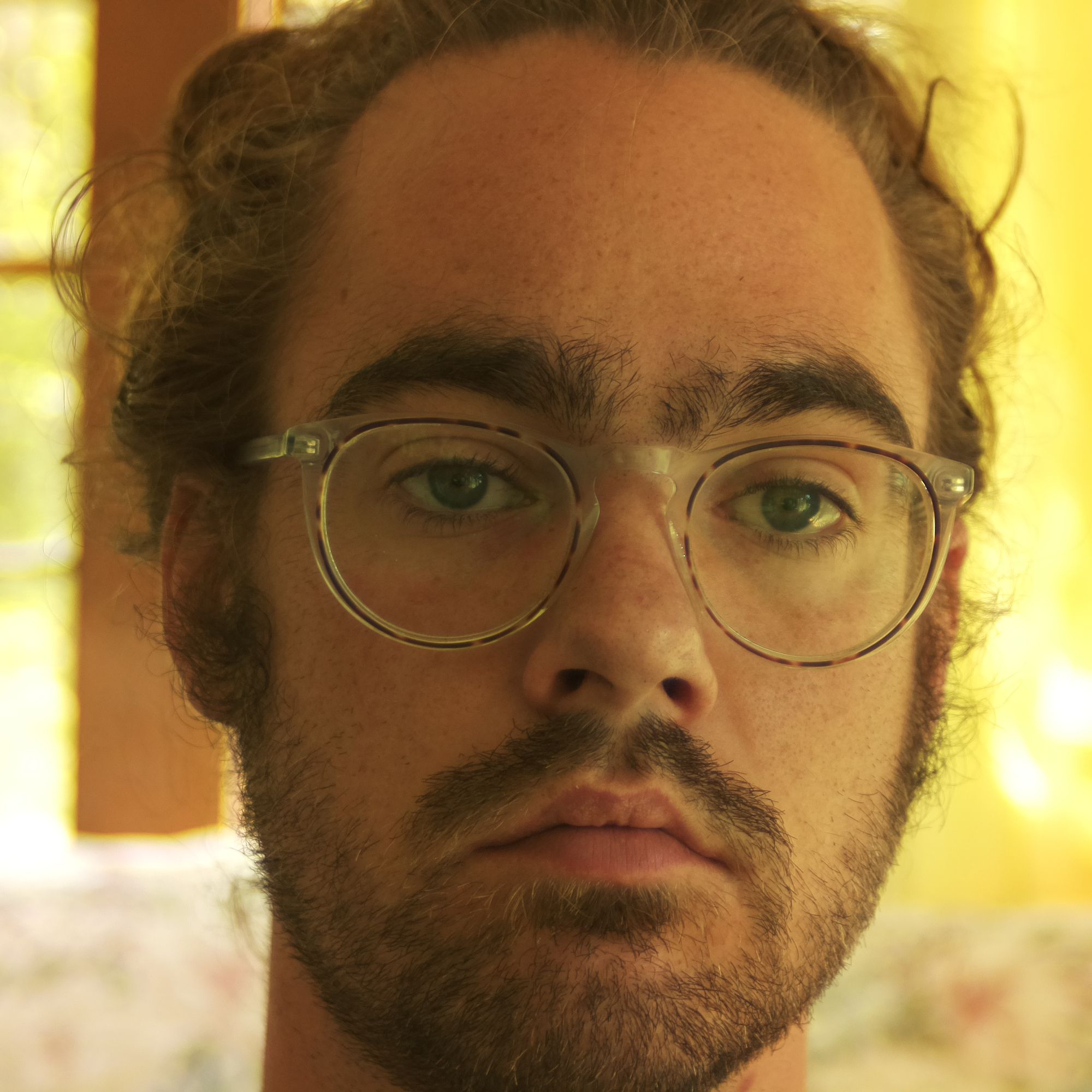
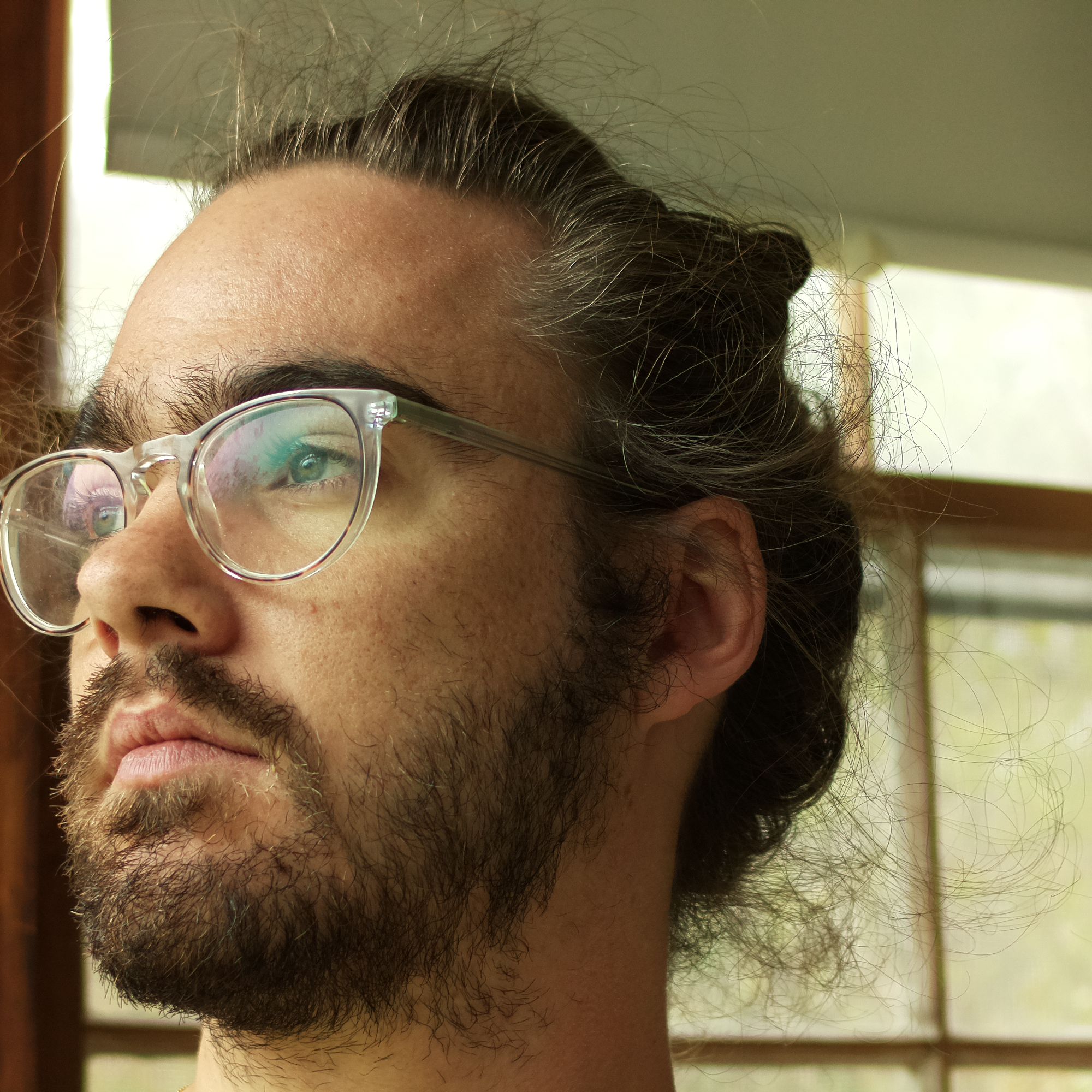
Having resolved to try and use this technology to create album art for the upcoming release, the first step was to take portraits of Won Pound, creating the most exhaustive photographic record of him in existence.

Capturing Images

Without any specific ideas of what the fruits of this project were going to be, it was decided that we would stay within the relatively safe harbor of portraiture. Focusing faces worked for Gwern and the original authors of StyleGAN. This meant that ‘portrait’ became the term-of-art to describe the images used in the training dataset. There are a few conflicting reports of just how many images you need to train a useful network. It’s not millions, but it was more than tens of thousands.

Hardware

Having recently folded a Raspberry Pi HQ Camera into my 3D printing work flow for timelapse photography I knew it was perfect for this application. The camera is capable of producing spectacular images, and because it’s a Pi, it’s trivial to add a big hard drive to hold the resulting images. The max resolution of 4056 x 3040 would also be more than adequate. The following is a photo of the setup used to capture the images for this project.

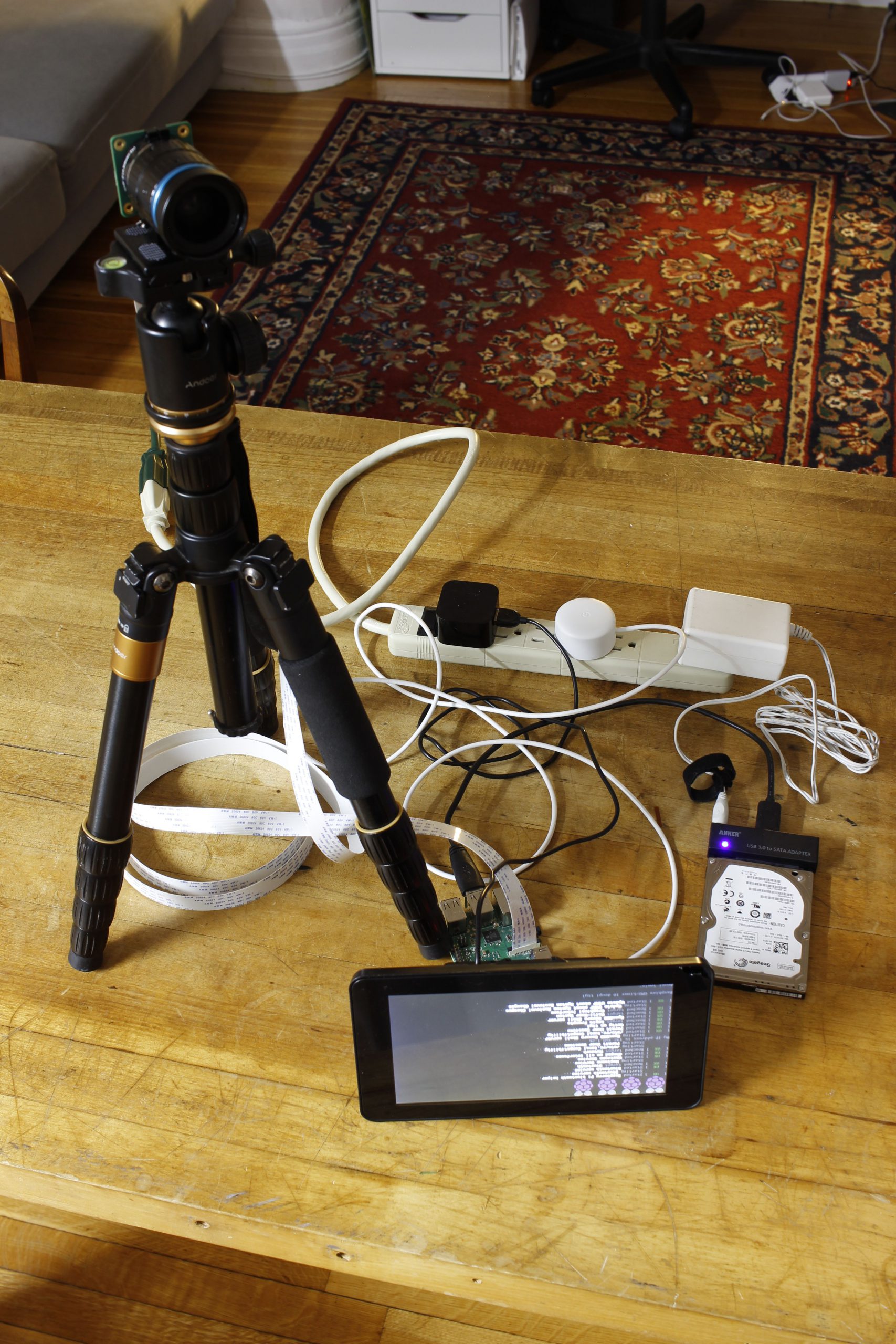
Raspberry Pi: Raspberry Pi 3 B+. Any Pi that supports the HQ cam should do, this is what I had on hand.

Display: Raspberry Pi Touch Display.

Storage: Samsung EVO 860 500GB SSD. There’s a USB 3.0 to SATA Portable Adapter used to interface with the SSD. This particular unit also has a 12V DC barrel jack input to make sure the hard drive’s power draw doesn’t overload the Pi’s power supply.

Camera: Raspberry Pi HQ Camera. An extended ribbon cable was also used to connect the camera to the Pi.

Lens: 16mm Telephoto Lens.

Tripod: Andoer 52 Inch Tripod. This is included to say that it would be very hard to take this many photos free hand.

Can’t say that I’m too proud of the free-form nature of this camera setup. Surprisingly we never really ran into issues with the hardware. Should the need come up to capture another couple thousand images I’d like to design a more monolithic housing for these components.

Software

The CLI to capture these images has been published on GitHub as pitraiture. It’s a thin wrapper around the picamera python package to add a few usability features. The main feature is that it will open a preview before staring to take photos.

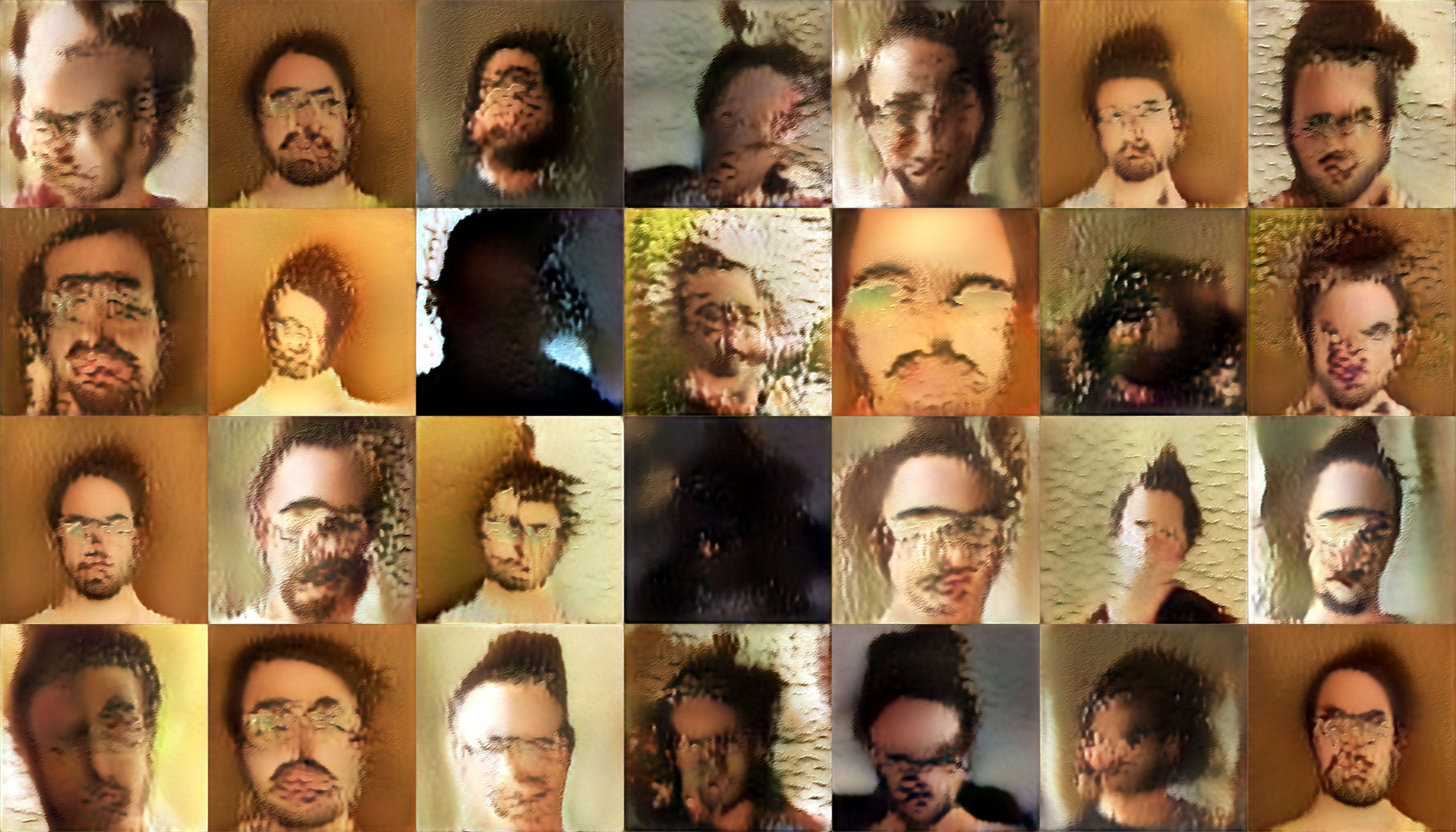
It took a few attempts to get a worthwhile training set. Initially we fell into the quantity trap, capturing thousands of poorly lit, out of focus shots of Won at work in his studio. The resulting images produced by networks trained on these portraits reflected the lack of intent here. Here’s a sample from the initial set:

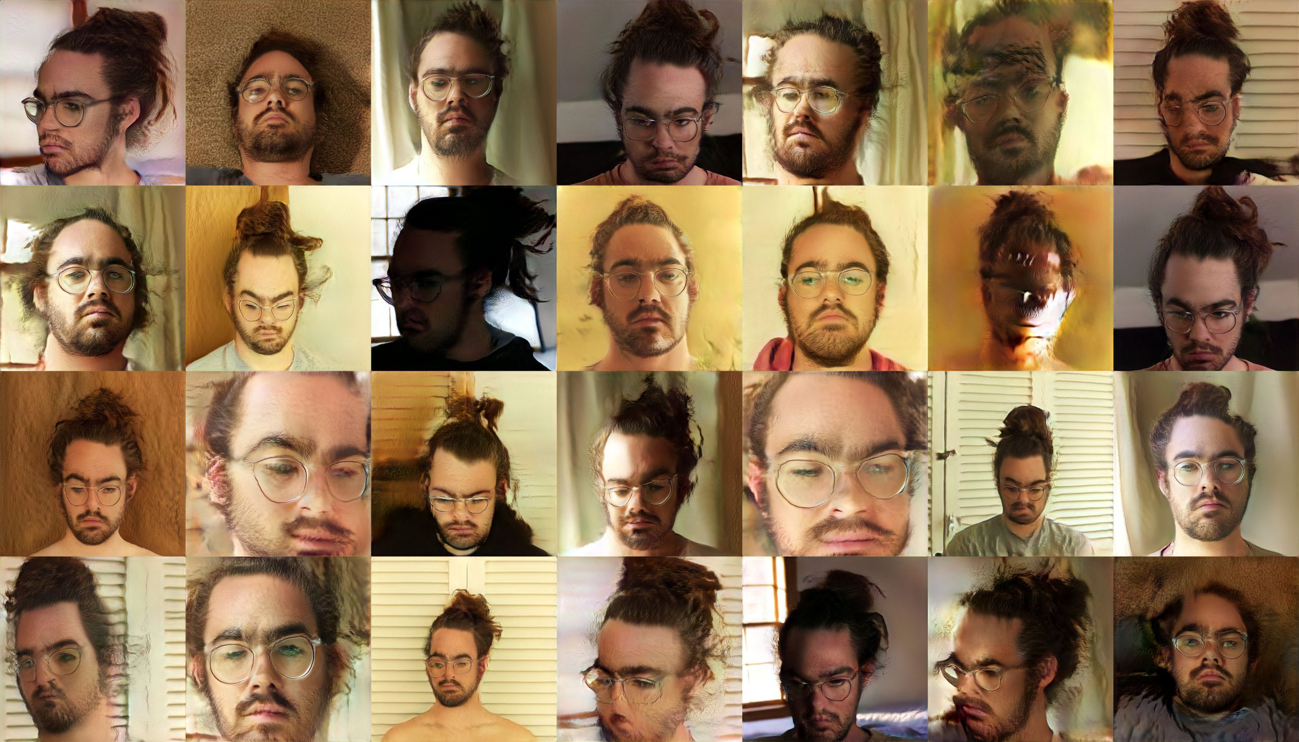
In the end, the strategy that prevailed was to take 2-3 thousand shots at a time, then change scenes. This was done around 40 times to get the final set of images.

ownCloud

Outside of dropping the camera off and picking it up months later, I personally wasn’t on site for any of the portraiture sessions. This lead to the small matter of transferring these files from his studio to my server (which lives in my apartment).

Pitraiture includes the ability to upload photos to my ownCloud instance once a session is complete. The Pi had an authenticated ownCloud client pre-installed, so this upload operation is implemented with a local copy, from the Pi’s SD card to an SSD that is monitored by the ownCloud client for files to upload. This was a quick and dirty, no-cost solution that served us well. The idea of having to manually move all these images makes me shudder.

Selecting good images

The raw dataset size was initially 77,224 images, but after some analysis with the face-recognition, and manually going through sessions that number was decreased to 50,000 of the best photos. Images were captured at a resolution of 2000 x 2000 but scaled to 1024 x 1024 for config-e training.

Training Networks Locally

Images in hand, it was time to get training.

This step in the process consumed the most amount of wall time, so I aim to be as concise and opinionated here as possible to hopefully save others some time.

To train the networks, I eventually settled on using config-e at near-default settings. Check out the training section of the Gwern post listed above for some explanation as to how the different training parameters effect the resulting networks. The images produced by networks with these near default settings looked totally adequate for the feel of what we were going for. Getting this to run at all was a bit of a process so I didn’t really explore tuning training parameters as much as I probably could have.

The final network we’ve been using for the production images took 72 days to train using a single GPU on an NVIDIA Tesla K80.

Working with GPUs

The production dataset of 50K images occupied around 48GB of space on disk. This ruled out many of the free cloud-based AI solutions that are out there (google collab, paperspace etc.) as moving this amount of data would take hours and hours, blowing through GPU allocation time.

Additionally, the idea of being billed for each hour I spent with a cloud GPU was worrisome. I’m self-aware enough to know that this would result in me frugally rushing to results rather than experimenting with the process. These considerations made me opt to complete training and the rest of development locally using mostly hardware I already owned.

Too slow to play games on, and too inefficient to mine cryptocurrency with, the NVIDIA Tesla K80 is a very cost effective way to get into AI research. As they’re a few generations old, they can be had for under $150 on ebay, while still boasting a total of 24GB of VRAM. This is perfect for config-e training. These cards are a rabbit whole of their own. They require ‘server motherboards’. The key BIOS setting that your motherboard must support is ABOVE 4G DECODING. The base address registry needs to be able to address the whole 24GB of VRAM on the cards.

So long as your hardware setup meets these requirements, you should be able to use the cards. Training and projection (which we’ll get into later) required a lot of memory, I’d recommend at least a 64GB kit of RAM. The rest of the host’s hardware config shouldn’t matter, and there are many examples of people using these cards online in a wide variety of builds.

If your motherboard doesn’t, meet these requirements, you may have a hard time finding out. lspci -vvv ended up being a favorite tool for working through these issues. You want to see outputs like:

Showing that the full range of memory can be mapped before trying to install the drivers. If you run into results like:

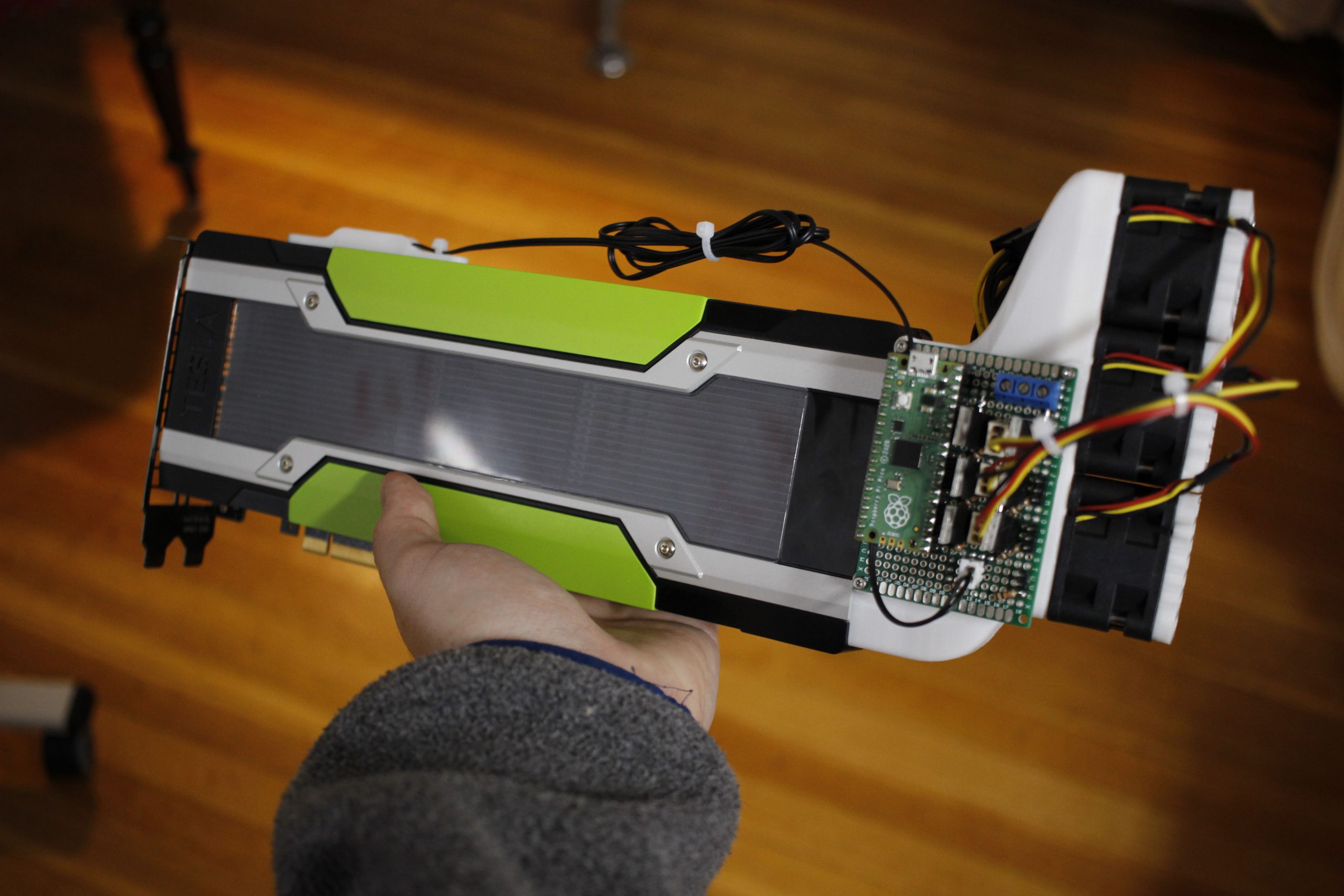
You might be out of luck. For what it’s worth, I also found that 100% of the time the GPU stopped responding was because it was too warm. These cards can put off an impressive amount of heat. To get around this, I developed and published an open-sourced GPU cooler specifically for these cards to service this project.

To train, inference, project and generally interact with the GPUs at all, the workflow I landed on goes something like this.

1. Use a runfile to download and install the drivers for the GPU.
2. Use docker-compose to stand up a docker container based on the Dockerfile published by NVIDIA.
3. SSH into the docker container and get to work on development / have the docker container run till it’s completed it’s work per the Dockerfile.

Using docker saves you the potential headache of having to debug a CUDA/nvcc installation. To actually run my code, I would most often use a pycharm remote interpreter linked with one of the GPU-enabled containers.

My GPU development environment

In the interest of knowledge sharing, the following section describes in detail the software/hardware setup I’ve been using throughout the development of this project. The only requirement to use GANce is to have a CUDA development environment with enough VRAM (as was previously described).

The server wasn’t purchased specifically for this project, I had been aggregating parts via eBay for some time before getting into this work. However, the GPU’s as well as the second CPU were additions made to service this project.

Software

The OS running on the server is Proxmox VE. I prefer to work on project development inside of VMs whenever possible. The benefits of total system backups and running snapshots outweigh the learning curve of getting things set up. SPICE, which is baked into Proxmox enables ultra low latency VNC access to VMs even through a VPN. My Macbook air an quickly transform into a workstation and all that is required is an internet connection.

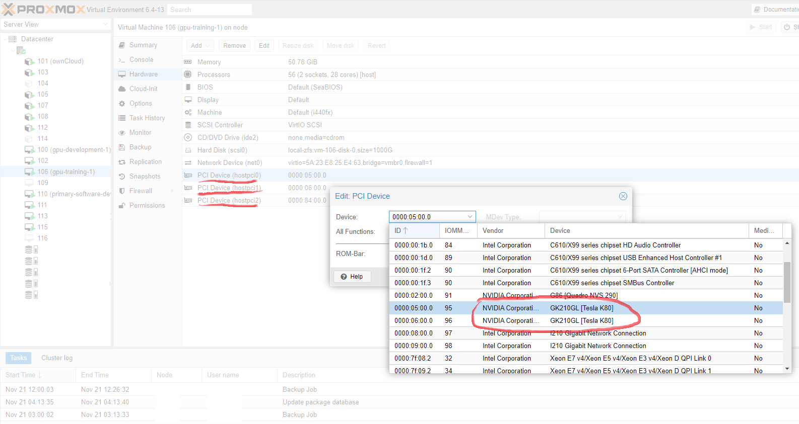
Proxmox is able to pass the GPUs into virtual machines with ease. Currently I have two VMs that get GPU access. One for ‘development’ and one for ‘training’ The development VM is for short term tasks that should complete quickly where as the training VM is for longer running tasks like projection or training.

Since there are two logical GPUs on a single K80, we can actually pass these individual cores into different VMs. The development VM gets a single GPU core and the training VM gets three.

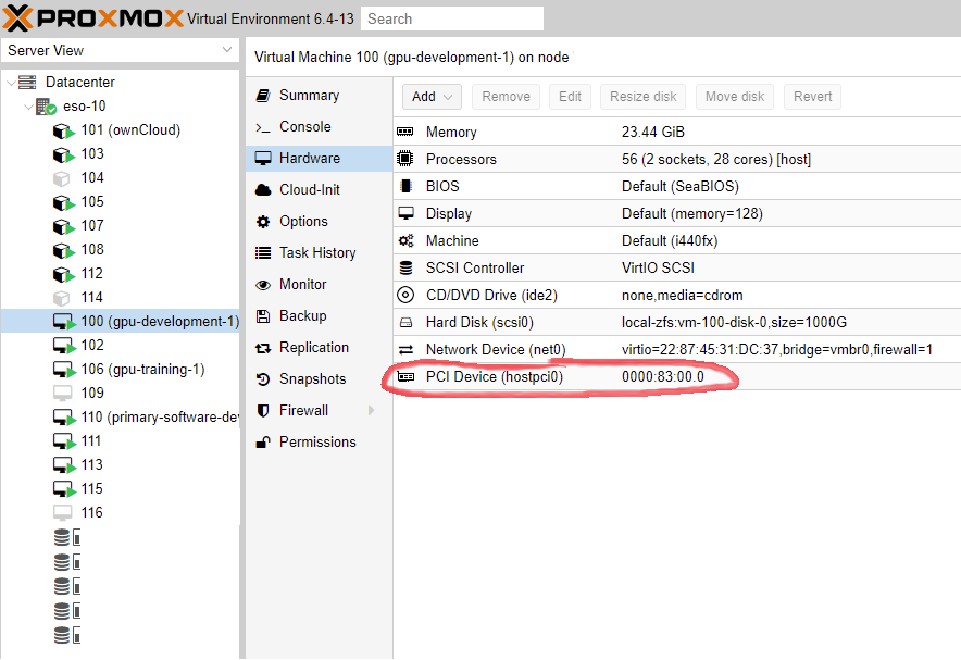
This enables a few cool development improvements like being able to totally power off a GPU core when it’s not being used.

Hardware

Motherboard: SUPERMICRO MBD-X10DAX-O. This is probably overkill, but it has enough headroom to be useful for years and years to come. There were a few BIOS tweaks needed to get all of the different components working, but those will be mentioned in their respective sections.

CPU: 2x Intel Xeon E5-2690 v4. Imagine my horror in discovering that in order to use all of the PCIe slots, both CPU sockets on the motherboard have to be occupied. Just kidding. While two CPUs were required, I was giddy, not horrified to fill the Xeon-shaped hole in my heart (and motherboard). 56 cores is a hilariously excessive amount of computer to have at one’s disposal.

Initially, after adding the second, CPU I was getting a QEMU error when starting the VM with one of the K80s GPU pinned to it. Something about a permissions. The proxmox documentation provided a path to a resolution:

I saw:

Then ran:

And things worked as expected after a reboot.

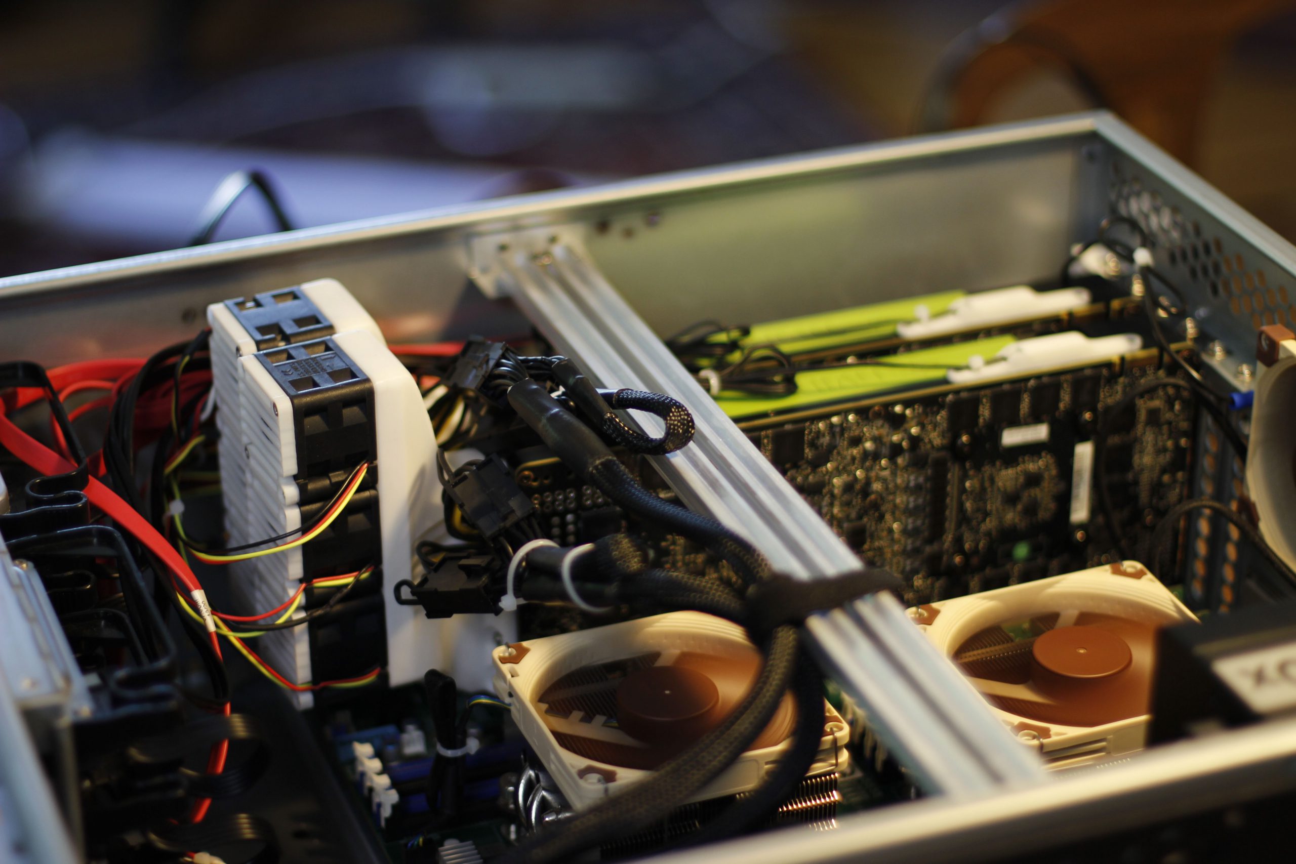
CPU Cooler: Noctua NH-L9x65. These are “low profile”, hopefully this will give me some flexibility down the line when it’s time to move these parts into another build.

Compute GPUs: 2x NVIDIA Tesla K80 with high performance coolers.

Initially upon installing the second K80, I found that I could see the device in Proxmox, and boot virtual machines with the GPU passed in, but actually trying to use the GPU would result in the dreaded No devices were found error from nvidia-smi. After doing a bit of reading in the manual, I adjusted these BIOS settings on my motherboard like so:

You’ll also want to enable persistence mode on the GPUs whenever possible to avoid confusion. There is some documentation out there around increasing the performance of these GPUs. However, it seems like the biggest boost can come from bumping up the max power draw to 175W. Your mileage may vary here, I didn’t really notice a significant increase in performance of projection or training after making this change.

Other GPU: HP NVidia Quadro NVS290 NVS 290 256M. This is an adorable, PCIe 1x graphics card that is passively cooled and can be yours for under $20. In this build it’s used to interact with the server directly using a keyboard and mouse.

Memory: 128GB (4x32GB) DDR4-2400MHz PC4-19200 ECC RDIMM 2Rx4 1.2V Registered Server Memory by NEMIX RAM. The order in which you install the individual sticks of memory into the server can impact their operating speed. Make sure to consult the docs for this. I also found that the memory was configured to run at 2133MHz by default. I had to manually increase this to 2400MHz in the BIOS.

Storage: The main storage pool consists of 4x Seagate Exos X16 14TB 7200 RPM SATA drives.

These are configured in a RAIDZ-1 (which is ZFS for RAID5). This means one of the four can fail and no data will be lost.

There’s also a 500gb Samsung EVO 860 SSD that houses the set virtual machines I interact with using mouse and keyboard. These need to be a little more responsive, and don’t need a direct line to the main storage pool.

Power Supply: Corsair RM850x 850W power supply. Haven’t run into any problems with this yet. By my math it might be possible that my peak power consumption could draw more power than this unit is capable of dispensing, but I haven’t run into that problem yet. Were I to build this out again however, I would use a 1000W PSU.

Case: Rosewill RSV-L4000U 4U Server Chassis Rackmount Case.

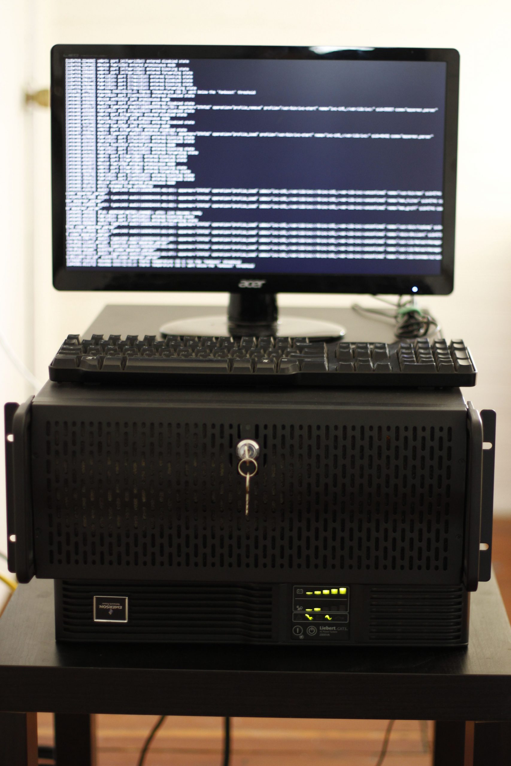
UPS: Emerson GXT3-2000RT120 2000VA 120V

While it is possible to recover from mid-run crashes of both training and projection, god damn does it feel luxurious to be imbued with the peace of mind that comes with a big beautiful UPS.

This one was purchased used on eBay. The fans were replaced with quieter Noctua models, and the batteries were replaced with, well, working batteries. There may be a blog post on this repair process in the future.

Synthesizing Images

Images captured, networks trained, and a development environment meticulously arranged, it was time to start playing with networks.

Each of the images and videos in subsequent sections were generated with GANce. There will either be an explicit CLI command listed, or you can look in the blog_post_media function of visualization_examples.py.

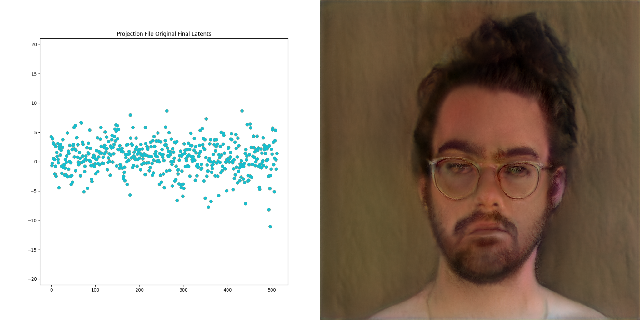
The key realization thus far is that the mysterious latent space is just a list of numbers. StyleGAN networks can be thought as black boxes that deterministically map lists of numbers into images. For the remainder of this post, the vectors on the left side are fed into the network to produce the resulting image on the right.

 

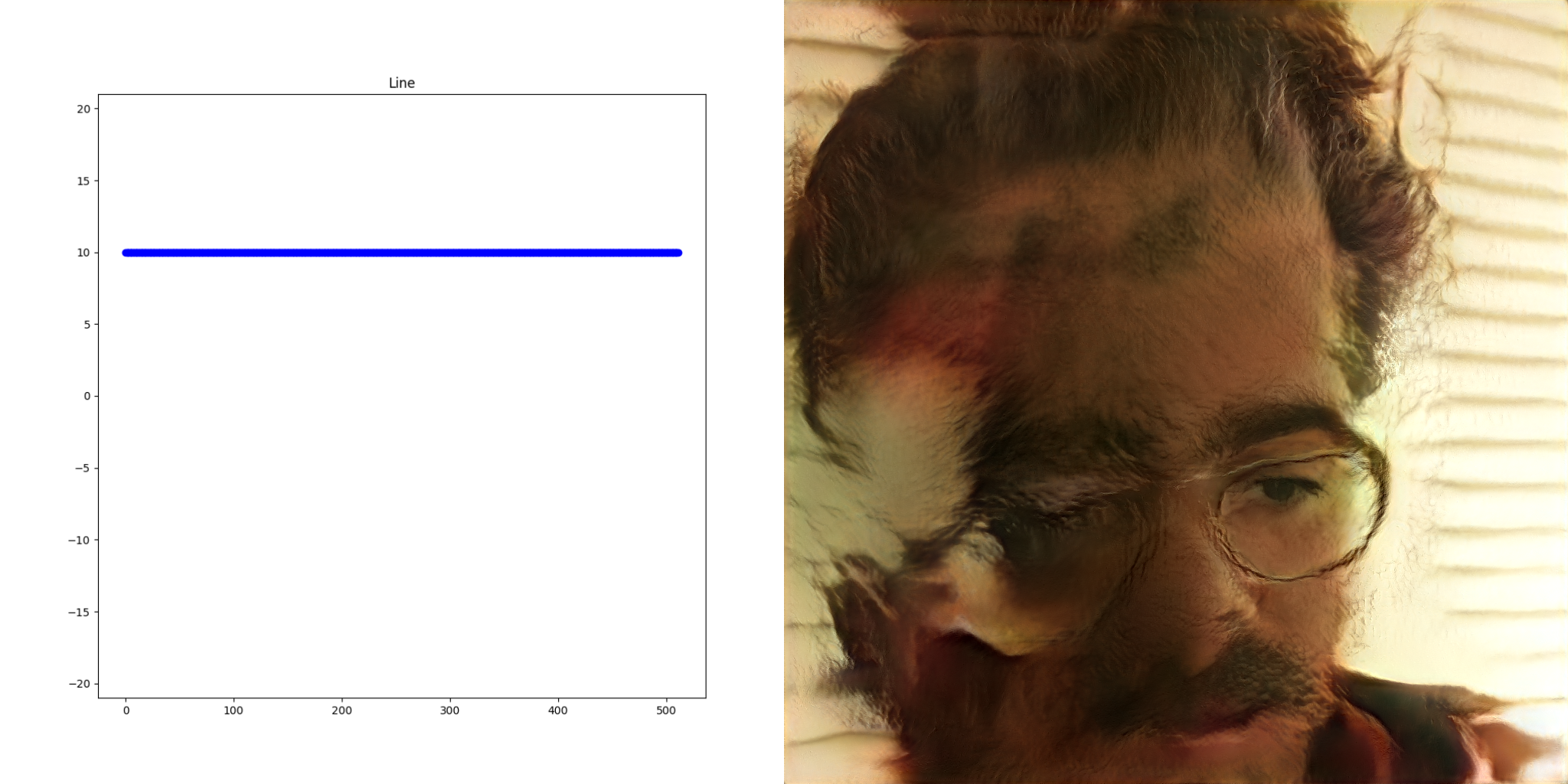
Extending the analogy, these black boxes also have the property that two lists of numbers that are similar produce images that look roughly the same.

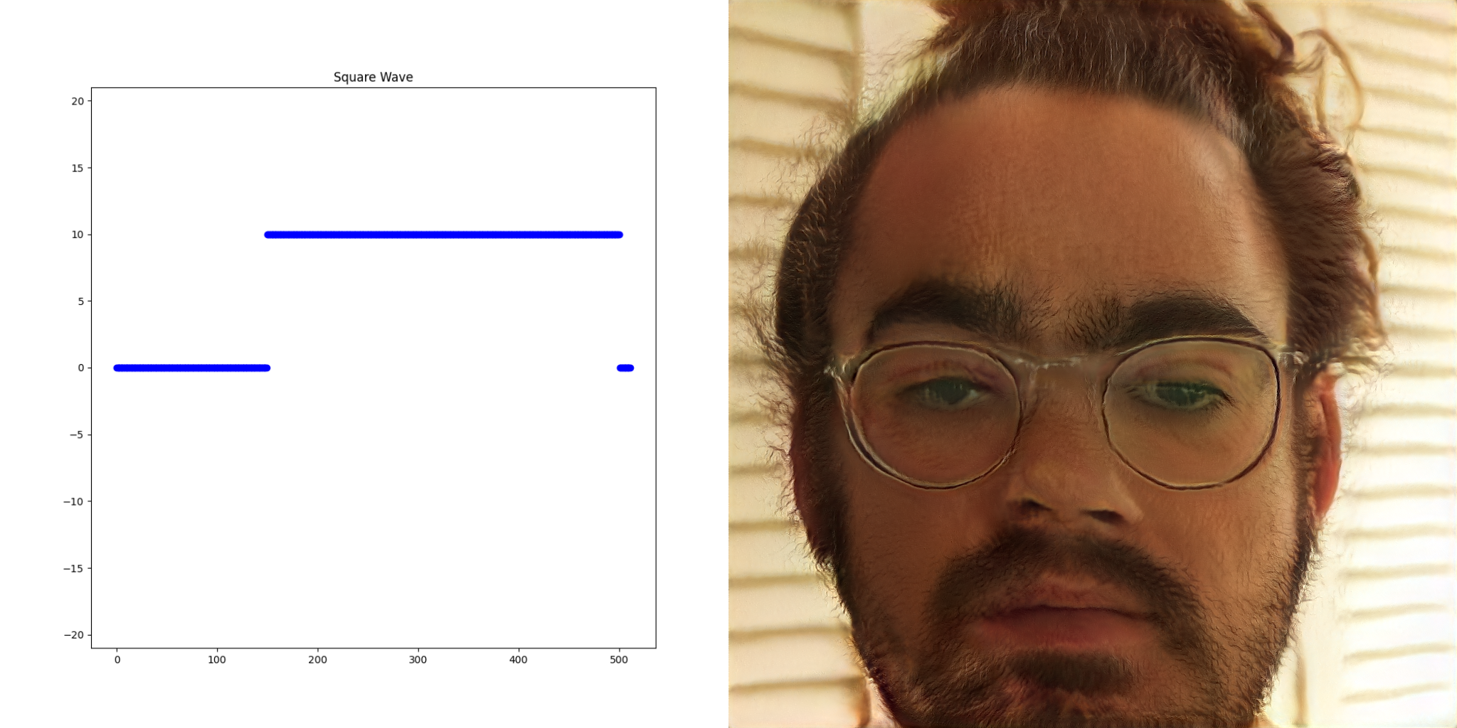
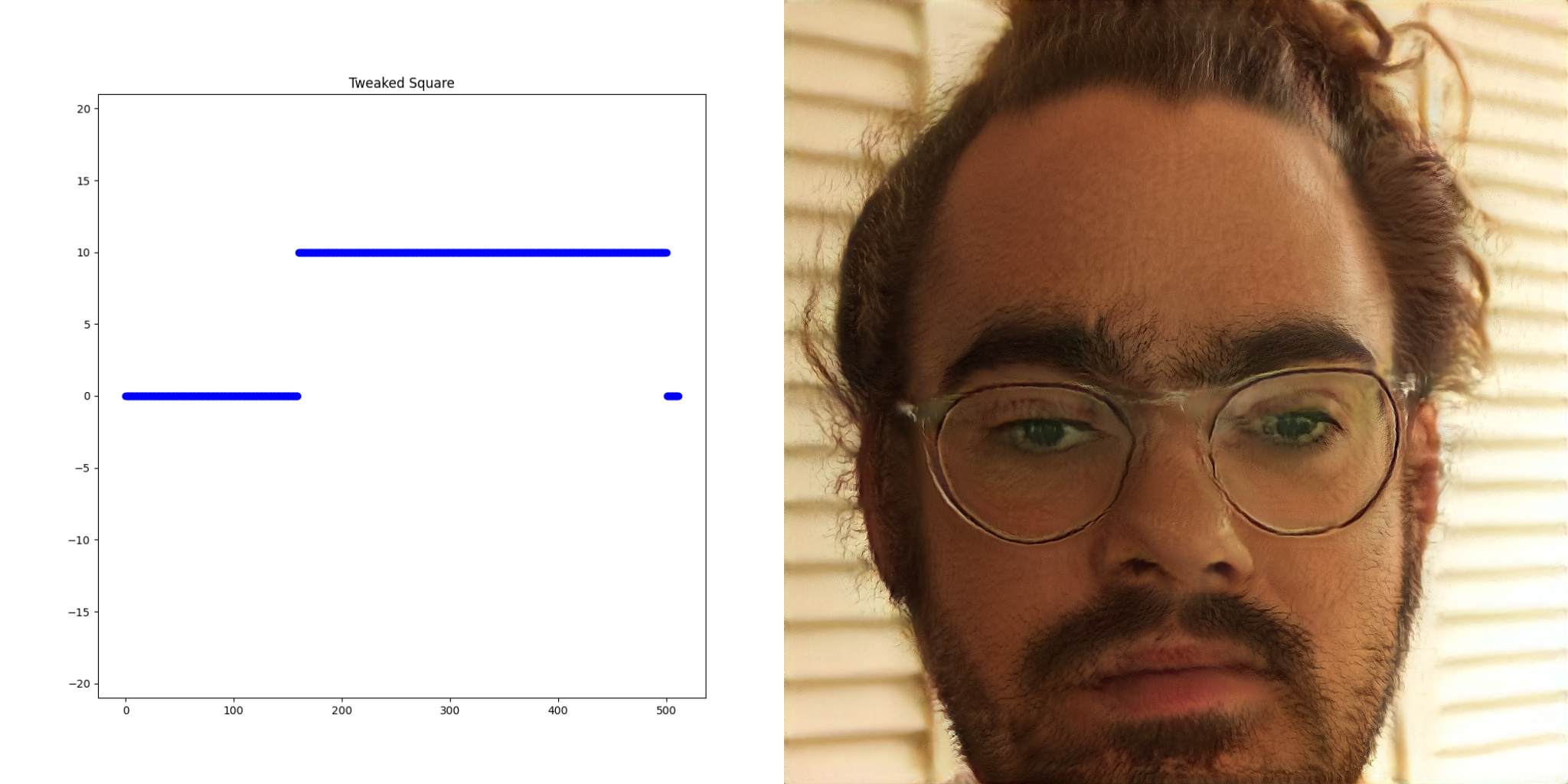
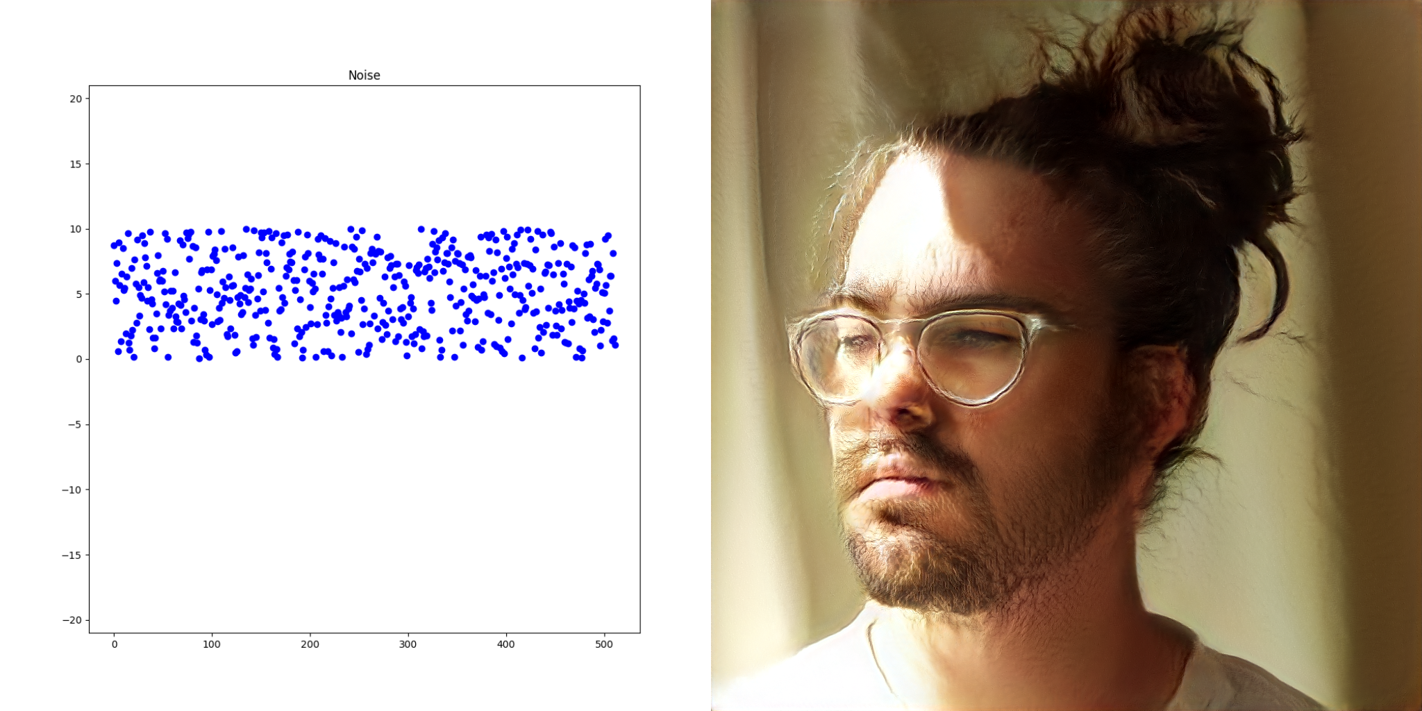
These properties were leveraged to create the static assets for the collaboration. Hundreds of images based on random noise were created. Each time one appeared that was interesting, the input vectors (a vector is just a list of numbers) were recorded and then tweaked to create even more images until the final album cover, poster etc emerged.

This property is also what enables smooth videos. Using interpolation, or gaussian blur, or a Savitzky–Golay filter, we can smooth together lists of lists of numbers and produce output images that are correspondingly smooth in their transition from one list to the next.

Adding Music

In our collective digital reality, almost anything can be thought of as lists of numbers including music. Music also has the similarity property described in the previous section; adjacent moments in a song typically sound alike. What would happen if a wav file was piped directly into the network?

If you watch enough times, you’ll start to see a whisper of reactivity between the music and the output video. Seeing results like this prompted me think about synthesizing entire music videos, not just still images.

After applying a few transformations on the music, and using alpha blending to combine the music with smoothed random noise, we can create some output that looks very interesting.

The top plot is the FFT, the second plot is the blurred noise, and the third plot is them combined with alpha blending. You can ignore the last three plots for now, those will be explained in the next section.

Network Switching

There is a third property of these networks that can also be leveraged. During training, networks are incrementally created. The process can produce hundreds of networks throughout the training process if desired.

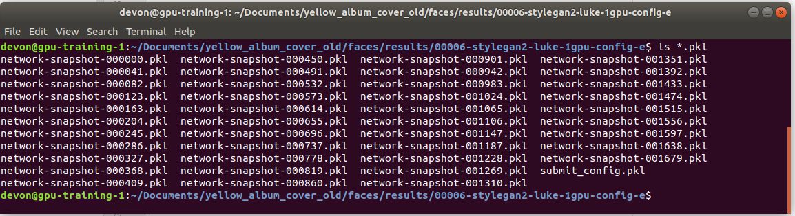
These are snapshots of the network as it’s trained. A network early into training is going to produce images that look less like the input dataset than a network that is deep into training.

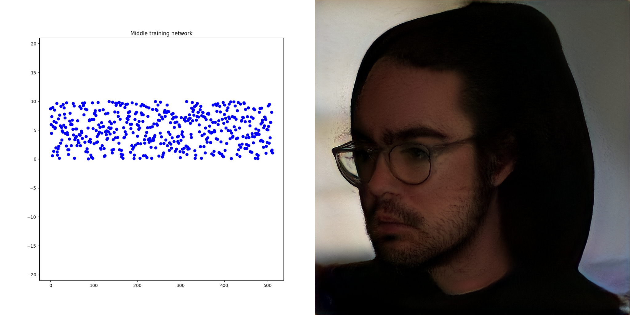
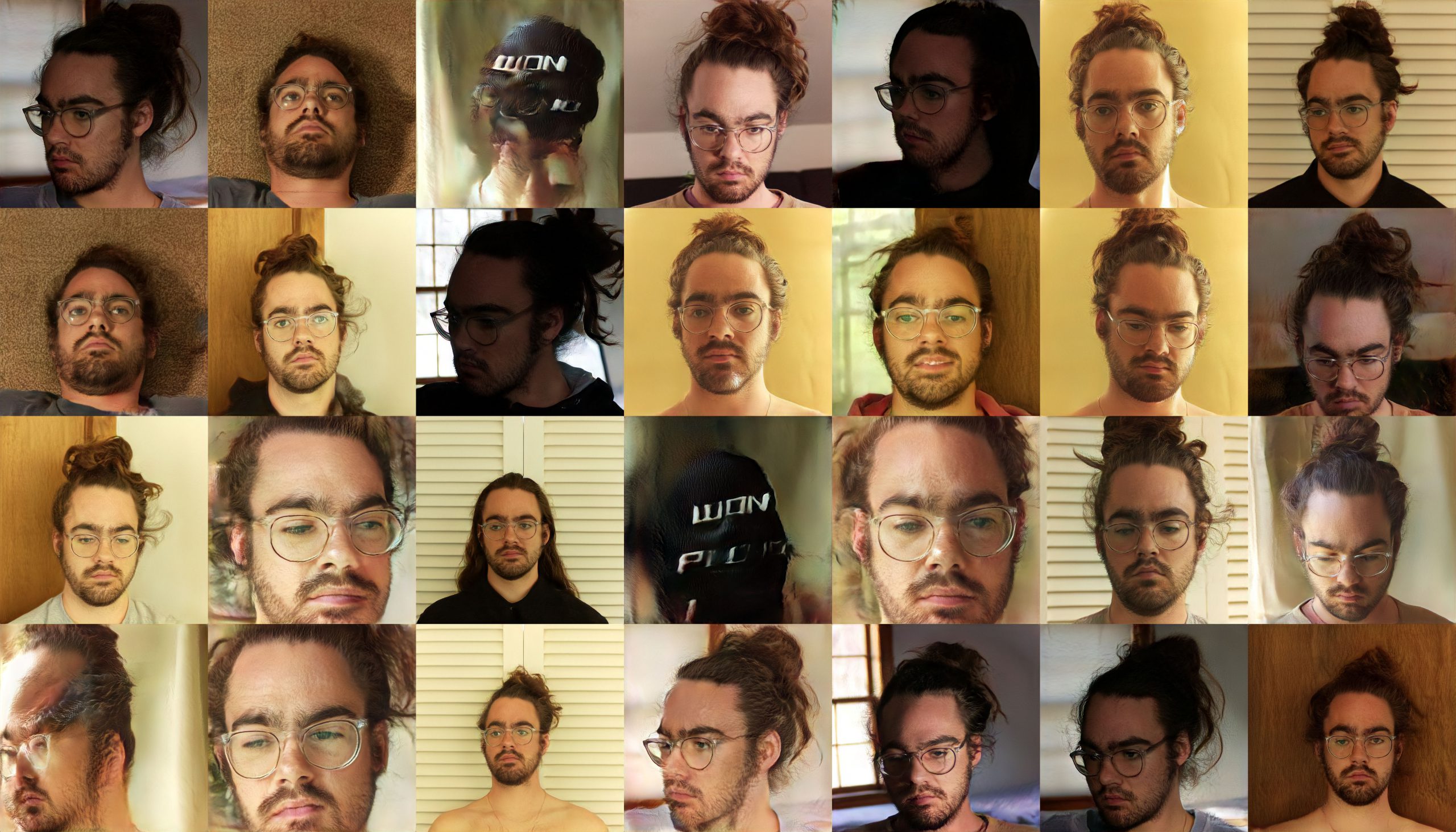
Turns out, if you feed the same vectors into multiple networks from the same training job, the results look visually similar. Earlier networks look less defined, later networks look more like the training images.

The result here is phenomenally cool. You can visualize the improvements in the training process.

This can be mapped to another parameter in the music videos as well. What if the complexity of the music defined which network was used? Mapping complicated moments in the song to well-trained networks, and quiet moments to early networks.

The bottom three plots are a visualization of which network index is being used. It shows the RMS power of the chunk of audio, with this then quantized into the range of networks we have to use. The final plot shows, for each frame, which network is being used.

This adds some variety to the videos, a bit more dynamic behavior. At this point in the development process I was somewhat happy with this result, but wanted to keep digging.

Projecting a video (projection file)

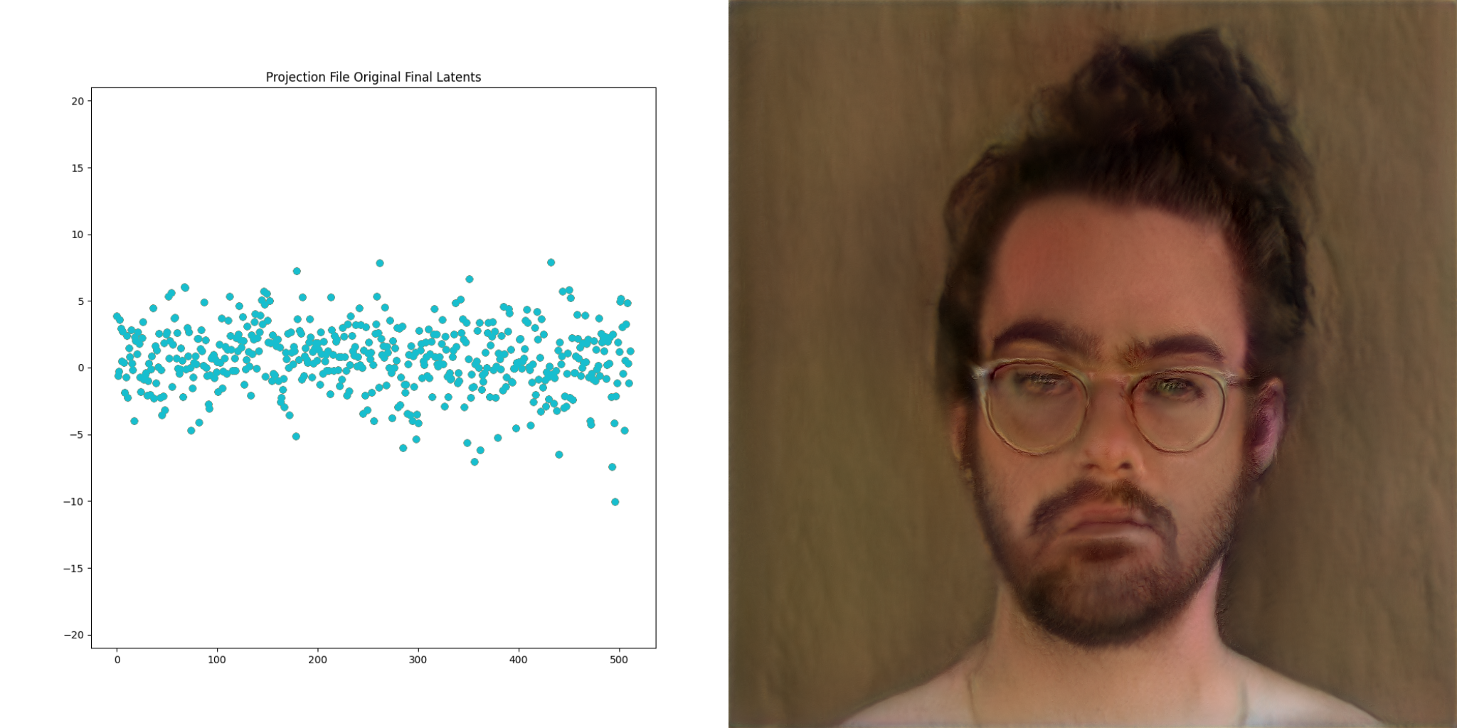
Up until now we’ve been talking about going from lists of numbers to images. StyleGAN2 also exposes a way to go the other direction. This process is called projection, because images are projected into latent space. Here is a visualization of this process:

The image on the far right is the ‘target’. The resulting vector is called the final latents, and is very interesting to consider. The second property above still holds. We can modify this slightly, just like can be done with the vectors in previous examples, and get a visually similar output

Video is just a collection of images right? What if we project frames of a video and then play the resulting images back at the same frame rate as the original?

This grants the ability to direct the network to produce the basis of an output video that we have complete control over.

The GANce repo introduces the concept of a projection_file, which is a way of storing the resulting final latents for each frame of a given input video. It also stores the projection steps along the way, as well as some other information. Projection files are just hdf5 files under the hood, which is a fancy way for storing… you guessed it, lists of numbers. There is a reader/writer for these files in the projection package within GANce, and there’s a few sample files in the test/assets directory as well.

It takes around 10 minutes to project a single frame using default settings, and the hardware setup as previously described. This means that you could quickly spend years projecting large, high FPS videos. There are a few ticks we can do to save time.

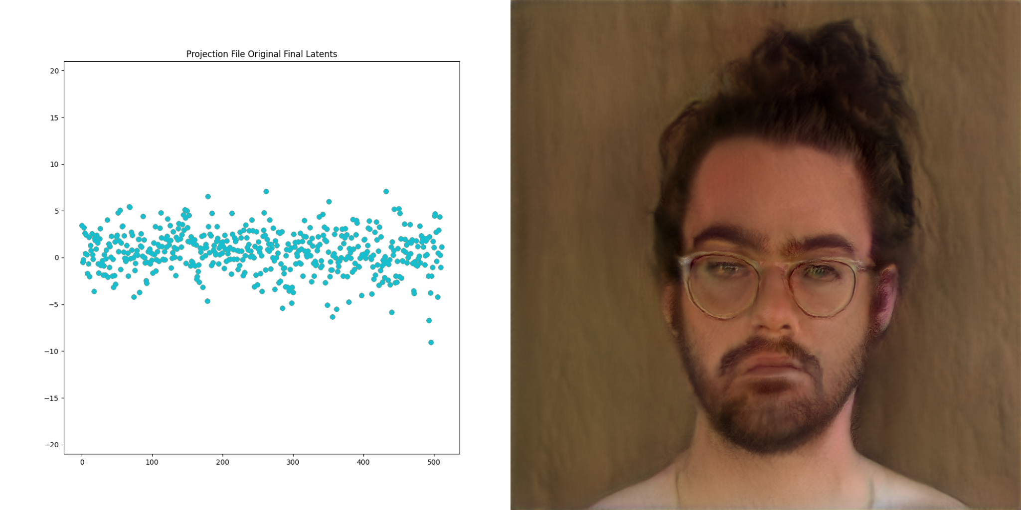
Projection steps are the number of images the network produces along the way toward the final projection. By default, this is set to 1000 in the StyleGAN2 repo. I’ve forked the repo to make this value configurable. Though experimentation, it’s clear that in our case, the full 1000 steps aren’t needed. Projecting each frame 607 steps resulted in vectors that were 80% completed. This completeness yardstick is the total difference between each point in the given step vs. it’s corresponding location in the final step. You can see this phenomenon visually:

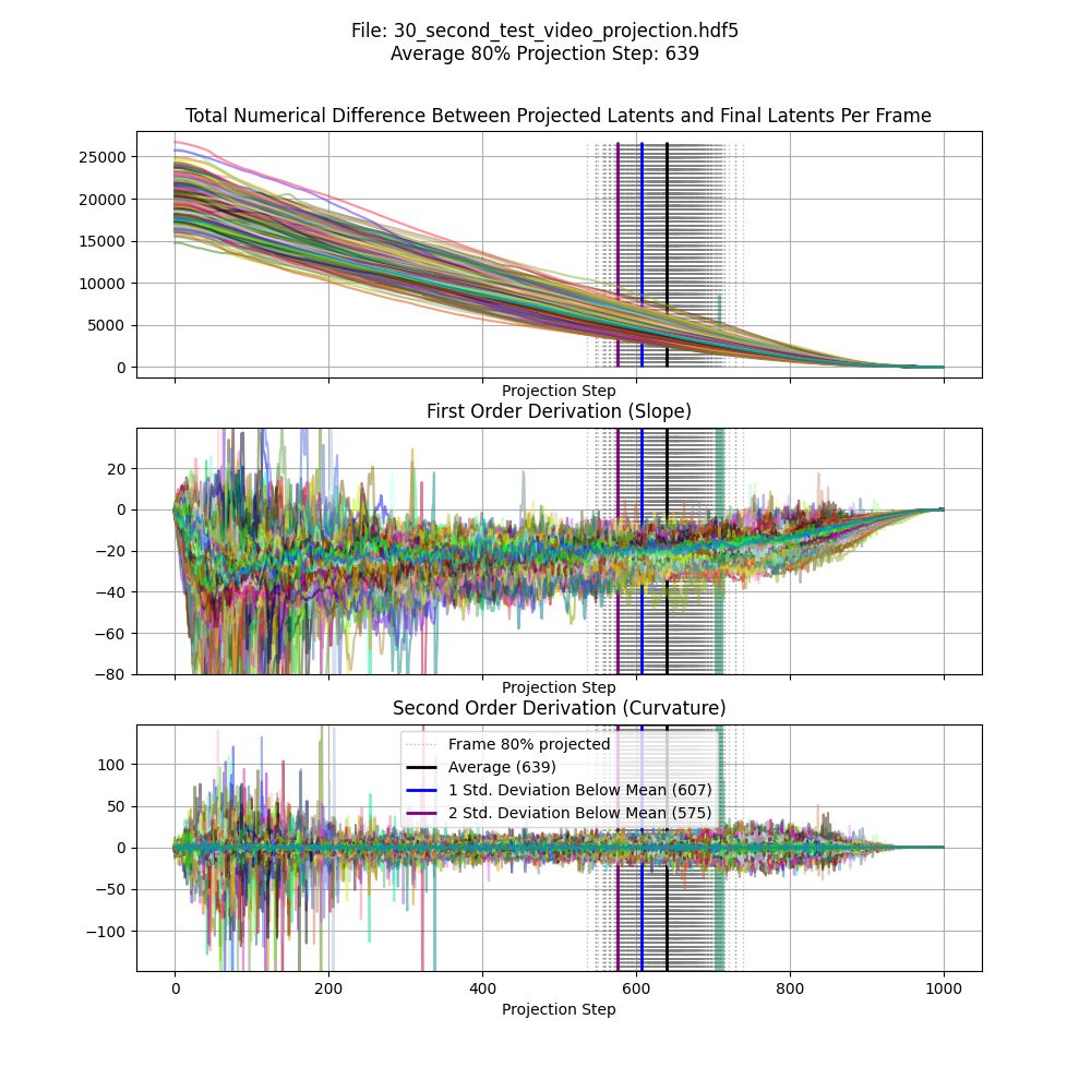
Apologies for the hand-wavy math, this is easier to see visually. In the projection example above, you can see how things settle in toward the end of the video.

The other time savings we can implement is to reduce the FPS of the input video. For this project, we found that 15fps produced very compelling video. We can use a couple of techniques to bring that 15FPS back up to 30 or 60. For this example we’re multiplying the frames. Each frame of the projection gets shown four times in the resulting video. Other inputs can be combined with the duplicated video latents to ensure that something unique is happening each frame, even if the primary source material is only 15FPS. Here as some visualizations of these different techniques:

 

You can also increase the amount of hardware you use to create these projections to save time. I ended up purchasing a second K80 for this purpose explicitly, projecting one video per core.

So, for an album 26 minutes in length, and a full-length video recorded at 15FPS, it took around 23 days to project the entire video. A long time but not completely unreasonable.

After all of this, we now have another list of numbers, this time one that represents a video. You can probably guess where we’re going next.

Music + Projection File

Instead of blending the FFT from the music with smoothed noise, what if the music was blended with the projected video?

Adding network switching back in and that concludes the progress I’ve made on this tool so far.

This is the stopping point for now as these videos hit the mark. The combination of musical input, network switching, and projection file input produces videos that are raw and evocative to match Won’s sound.

Future plans

The pipeline to go from time series audio to resulting images is, at is stands, optimized for correctness and readability without a thought at all given to performance. As it stands though, images can be synthesized at an unexpectedly fast 9FPs.

This opens the door to integrating this technology into a live performance. This is what is on the road map for development, maybe I’ll pick VisPy back up. These visuals would fit in just fine at a re;sample show.

Thanks for reading.